Overlay two heatmaps in R

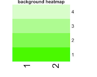
To-do: two heatmaps on two data sets with same dimension, overlay one over the other. For example, you have now heatmap 1 and 2 like these (generated in R, dataset is 4 by 2). How to overlay red one on top of the green one?


Well, I really hope this problem is as easy as overlay two pieces of paper. Unfortunately there are a few extra miles to go. The steps are clear though:

1. get the rgb number on the corresponding position for paint and background heatmap, regardless of the values in the dataset
2. merge two rgbs cell by cell
3. plot the result rgb color matrix.

Before that, understanding how R assign colors to data from a color list, is needed. I actually played with some toy datasets and color list. Then I found that R will arrange data from smallest to biggest, and then assign colors according to the rank, so that the smallest and biggest will get the beginning and end of the color list. Say you have color c1 to color c8, and your ranked data set is (1,2,3,4). R will assign color c8 to 4, color c1 to 1. Color b and c will get in this case get color c3 (ceiling ((2-1)/(4-1)*8) and color c6. Thus given the color list a heatmap uses and the dataset that's been plotted, one can calculate which color is used to plot which data point. Well, I wrote a R function to accomplish this

heatmap_col <- function(val_array, col_list) {

minv = min(val_array)
maxv = max(val_array)

out = val_array
for( i in 1:nrow(val_array))
for( j in 1:ncol(val_array))
# take max of 1 or the other value in case 0 is the ceiling result
out[i,j] = col_list[max(1, ceiling((val_array[i,j] - minv) / (maxv - minv) * length(col_list)))]

out
}

With this then, I can easily get the rgb used on each cell of the heatmap. However, the returns are simply rgb code, like '#FF000045'(red,green,blue,alpha). We need to know the exact numbers of red, green, blue and even alpha, which are critical for the blending. After some serious googling, I found this colorful presentation very helpful. It contains a hex constant table, which could be used to break down rgb color into 4 numbers between 0 and 1, corresponding to red, green, blue and alpha. R code is here

hex_constant = data.frame(hex=c(seq(from=0, to=9, by=1), toupper(letters[1:6])), decimal=seq(from=0, to=15, by=1), stringsAsFactors=F)


rgb2hex_number <- function(x, hex_constant){

num_collector = hex_constant$decimal[hex_constant$hex == toupper(substr(x, start=2, stop=2))]
for(i in 3:nchar(x))
num_collector = c(num_collector, hex_constant$decimal[hex_constant$hex == toupper(substr(x, start=i, stop=i)]))

R = (num_collector[1]*16+num_collector[2])/255
G = (num_collector[3]*16+num_collector[4])/255
B = (num_collector[5]*16+num_collector[6])/255

with_alpha = ifelse(nchar(x) > 7, TRUE, FALSE)

if(with_alpha) {
A = (num_collector[7]*16+num_collector[8])/255
return(c(R, G, B, A))
} else { # fill in alpha of 0
return(c(R, G, B, 0))
}
}

The next step is to merge two rgb numbers on the same position. Two stackoverflow posts (here and there) talked about how to do it in python. If one happens to look up in wikipedia, one has to be skeptical with it.
Wiki is wrong about the operation could be associative. It's actually not, meaning switching background and paint colors while blending can yield different color. A quick algebra is enough. The R code for this step is trivial.

mix_2rgb <- function(x, y){
# x is the paint color, y is the background color
# NOTICE: this operation is not associative. Switching x and y may yield different result.

# lookup table of hex and decimal
hex_constant=data.frame(hex=c(seq(from=0, to=9, by=1), toupper(letters[1:6])), decimal=seq(from=0, to=15, by=1), stringsAsFactors=F)

# belending two rgb colors evenly
x_out = rgb2hex_number(x, hex_constant)
y_out = rgb2hex_number(y, hex_constant)

# with alpha channel considered
ax = 1- (1 - x_out[4]) * (1 - y_out[4])

if( ax > 0 ) {

rx = x_out[1] * x_out[4] / ax + y_out[1] * y_out[4] * (1 - x_out[4]) / ax
gx = x_out[2] * x_out[4] / ax + y_out[2] * y_out[4] * (1 - x_out[4]) / ax
bx = x_out[3] * x_out[4] / ax + y_out[3] * y_out[4] * (1 - x_out[4]) / ax

return(rgb(rx, gx, bx, ax))

} else {

rx = (x_out[1] + y_out[1]) / 2
gx = (x_out[2] + y_out[2]) / 2
bx = (x_out[3] + y_out[3]) / 2

return(rgb(rx, gx, bx))
}
}

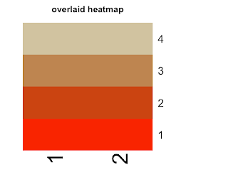
The last step is a little bit tricky. Since all I have for now is the colors I want to plot at each cell, but I don't have a data matrix to pass to "heatmap" function. So I have to do a hack using "rect" function. Anyway, This is the end result. Not bad, huh?

A Few Things Learned on Hadoop Streaming

In the past couple of days, I tried to run some map-reduce jobs on EMR through python streaming. The API I used is boto. It's really basic and not very documented. I was only able to find one example. One thing I learned the hard way is about the data coming out of hive. Surprising, no matter what input format (in terms of separators), the data out of hive is always 'ctrl-A' separated. Check this.

One-linear R: multiple ggplots on one page

First, par(mfrow=c(nrow,ncol)) does not go together with ggplot2 plots. Too bad, the simplest way I know of just wouldn't work.

There are two solutions I found out. The first is posted here. It's a smart function that performs par(mfrow) tasks. I just copied the code here

# Source: http://gettinggeneticsdone.blogspot.com/2010/03/arrange-multiple-ggplot2-plots-in-same.html

# Function used below in the function 'arrange'
vp.layout <- function(x, y) viewport(layout.pos.row=x, layout.pos.col=y)

# Function to plot multiple ggplots together
arrange <- function(..., nrow=NULL, ncol=NULL, as.table=FALSE) {
dots <- list(...)
n <- length(dots)
if(is.null(nrow) & is.null(ncol)) { nrow = floor(n/2) ; ncol = ceiling(n/nrow)}
if(is.null(nrow)) { nrow = ceiling(n/ncol)}
if(is.null(ncol)) { ncol = ceiling(n/nrow)}

## NOTE see n2mfrow in grDevices for possible alternative
grid.newpage()
pushViewport(viewport(layout=grid.layout(nrow,ncol) ) )
ii.p <- 1
for(ii.row in seq(1, nrow)){
ii.table.row <- ii.row
if(as.table) {ii.table.row <- nrow - ii.table.row + 1}

for(ii.col in seq(1, ncol)){
ii.table <- ii.p
if(ii.p > n) break
print(dots[[ii.table]], vp=vp.layout(ii.table.row, ii.col))
ii.p <- ii.p + 1
}}}

Another solution would be to use the 'grid.arrange' function in 'gridExtra' package. This function cooperates with not only plots, but also tables ('tableGrob'). So a plot can have both plots and text tables in it. And it has more controls over the title and sub titles. Very slick!

# Test
x <- qplot(mpg, wt, data=mtcars)
y <- qplot(1:10, letters[1:10])
arrange(x, y, nrow=1)
grid.arrange(x, y, ncol=1)

Use LDA Models on User Behaviors

LDA (Latent Dirichlet Allocation) model is a Bayesian statistical technique that is designed to find hidden (latent) groups of the data. For example, LDA helps to find topics (latent groups of individual words) among large document corpora. LDA is a probabilistic generative model, i.e., it assumes a generating mechanism underneath the observations and then use the observations to infer the parameters for the underlying mechanism.

When trying to find the topics among documents, LDA makes the following assumptions:

• ignoring the order of words, documents are simply bags of words and documents exhibits multiple topics.

• topics have distributions over words. So each word could appear in all the topics with different probabilities though. Say "transmission" will have a higher probability in the topic about auto repair, but lower probability in the topic about child education.

• each document is obtained by choosing some topics proportions, say {(topic A: .55), (topic B: .20), (topic C: 25)}.

• and for each word inside a document, choosing a topic from those proportions (say you randomly got number .6 (between 0 and 1 of course), the topic got chosen is B) then looking at the topic over words distribution and drawing a word from that topic (say word X).

Only the actual words are visible to us, so inference has to be made on per-word topic assignment, per-document topic proportion and per-corpus topic distribution. Dirichlet distributions are chosen to be the prior distributions for the latter two distributions. And various algorithms are used to make the inference, like Gibbs sampling (implemented in R package 'topicmodels').

LDA assumes a fixed number of topics existing in a document corpora and assigns soft membership of the topics to documents (i.e, a topic could be exhibited in multiple documents). Indeed, LDA is under a bigger umbrella called "mixed membership model framework" [refer to source [1] for more) .

The soft assignment and mixed membership nature of LDA models make it a reasonable candidate for user behavior analysis, particularly user behavior through a certain period of time. Say one has a log of user behavior at different stage of user life cycle (1st day, 2nd day, etc of a user's life). Then one can treat behavior as words, each day's users aggregated behavior log as document, and let LDA figure out the topics (group of behaviors that tend to appear together, 'co-appearance') and the proportions of the topics. And that will give some idea on how behavior of the group evolves over time. A R visualization could look like this (each tick on the y axis represents a topic).



However, I do find that sometime LDA tries too hard on discovering topics with niche words (after filtering out stop words and rare words). Depending on application, this could be a bless or a curse.

sources:
[1] http://www.cs.cmu.edu/~lafferty/pub/efl.pdf
[2] http://videolectures.net/mlss09uk_blei_tm/
[3] http://cran.r-project.org/web/packages/topicmodels/index.html
[4] http://www.cs.princeton.edu/~blei/

One-linear R: neat way to slice the data

Recently found out that library 'caret' has a few interesting functions, which are very handy to do the following tasks:
series of test/training partition (createDataPartition function)
create one or more bootstrap samples (createResample function)
split the data into k groups (createFolds function)

'Caret' is a super wrapper package. One can run different type of models by calling functions in this package only.

One-liner R: remove data frame columns by names

Sometime, I want to remove some columns from my data. What I did in that case, is found out what are the unwanted column ids and removed those. It's just a couple of lines in R. But why not write a function to do the job and also some error handling. So next time, I just copy and paste!

rm.col.by.name <- function(dat, colname.list){

l1 = length(colname.list)
l2 = which(colnames(dat) %in% colname.list)

if(length(l2) == 0) {
    warning('Did not find any matching columns. Check input column names, please.')
}

if(length(l2) > 0 & length(l2) < l1) {
    warning('Did not find all matching columns. Only those found are removed.')
    return(dat[,-c(l2)])
} 

if(length(l2) > 0 & length(l2) == l1) {
    return(dat[,-c(l2)])
}

}

Canopy Clustering

Lately I was introduced to a clustering algorithm called "canopy clustering". In plain English, like all other clustering techniques, it is designed to divide observations into segments (subsets, clusters, groups, buckets, whatever you call it), so that observations inside each segment are "similar" in terms of certain measurement criteria. Those criteria are distances or dissimilarities.

There are a lot of algorithms that cluster observations. Some are more computation-intensive, like k-medoids (compared to k-means). Some yield hard assignment, i.e., one observation can only belong to one cluster. Some generate soft assignment, i.e., one observation can belong to multiple clusters, like LSH (locality sensitive hashing) and canopy clustering. Some scale better than others.

Canopy clustering procedure is relatively straightforward. The key ingredients are two distance thresholds T1 and T2, where T1 > T2. For a list of data points, if a point is within T2 distance to any of the existing canopy centers, then that point cannot be a new canopy center; otherwise, it should be added to the canopy center set. With this rule, a set of canopy centers are obtained. Then if any of the input data points is within T1 distance of the existing centers, then the point belong to the canopy formed by that center. As one can see, a data point could belong to multiple canopies. The following plot illustrates the concept.



Usually, canopy clustering uses "cheap" distance metrics (easy and fast to calculate). So the process takes shorter time compared to k-means clustering. This is a typical trade-off between precision and speed. Thus people combine k-means and canopy together to cluster huge amount of data. The way the two works together is:
1. Canopy uses cheaper distance metric (however in the same direction of k-means distance, meaning if two points are close in terms of k-means distance, they should be close in terms of canopy distance too.), and partition data into canopies.
2. K-means still try to cluster all the data points, however distance between an input data point and any k-mean centroid is calculated if and only if they are in the same canopy. In this way, a lot of "unnecessary" calculations are avoided.

There are some interesting variations around combining those two or simply use canopy clustering to generate k-means initial centroids. If serving canopy clustering as a k-means centroid feed, one can only perform the center generation part, or perform both the center generation and membership assignment parts, and then re-calculate the center of the canopy clusters. If utilizing canopy clustering to partition the data for k-means first, keeping the ratio between number of canopies and k to 1 and 10 has been suggested. That means you always want the number of canopies be smaller than k. So that each point is likely to be in the cluster with at least one k-mean centroid. But how to find out how many canopies you are going to get? The trick is you have to play with T1 and T2.

When implementing in map-reduce framework, this blog post is very clear. One thing that is worth pointing out is that after canopy centers are generated using one map-reduce job, the next map-reduce job is to assign membership of all the input data to the canopy centers, at that time, some data may no longer be within T1 of any canopy centers, solutions in this case includes forming a new canopy with this point as center or assigning it the nearest center or simply discarding that point.

A few things I learnt in 2010

2010 was an "interesting" year. I write down the lessons that I learned and felt the most.

1. "Be confident and assertive."
Fine, call yourself "data analyst", "data scientist" or even "data ninja". Whatever you call yourself really does not matter. It matters that as a professional personnel, you work in an environment that requires you (and hopefully you would like also) to share your findings and convince others to see the potential value of your analysis the way you see them. At the end of the day, you are a consultant. And as a consultant, being confident and assertive about your expertise and findings help "tons" in the process.

2.Ask a lot of questions. Especially ask the "dumb" ones at the beginning. Getting clear on concepts and terms as early as possible helps reducing confusion and shortens project development time.

3.Follow up. Sometime people forget what they said or asked for a few days ago. Reasonably constant and consistent contact is the key to keep projects running and in track! Plus, it makes your clients feel needed, which theoretically is a good feeling. :P

Filesystem Traversing with Python

Lately I have accumulated a lot of files, most of which are papers in pdf format. Although they are put into folders properly, it's still hard to track down a single file, or even to check whether I have already collected that paper or not. So I needed to do a simple filesystem traversing and figure out 4 basic things about my documents: directory, file name, size of file, and last modified date. With a summary file that containing those information, I can do some kind of basic search, which is at least faster than my going through folders and digging files.

Also I wanted my results to satisfy two requirements (1) only output file information, if that file is in pdf, ppt, or doc format; (2) the size of file should be in meaningful format. I chose Python to finish this little task. Here is the code I used

import os
import time, stat 
from datetime import datetime

def sizeof_fmt(num):
    for x in ['bytes','KB','MB','GB','TB']:
        if num < 1024.0:
            return "%3.1f%s" % (num, x)
        num /= 1024.0

f = open('output.txt', 'w')  
  
for root, dirs, files in os.walk('E:\my_papers'):  
    for file in files:  
        if file.split('.')[-1] in ('pdf','ppt','doc'):
            st=os.stat(os.path.join(root,file))
            sz=st[stat.ST_SIZE]
            tm=time.ctime(st[stat.ST_MTIME])
            tm_tmp=datetime.strptime(tm, '%a %b %d %H:%M:%S %Y')
            tm=tm_tmp.strftime('%Y-%m-%d')
            sz2=sizeof_fmt(sz)
            strg=root+'\t'+file+'\t'+tm +'\t' + sz2 +'\n'
            f.write(strg) 

The modules that are used here are "os", "time", "stat" and "datetime".

First there is a user-defined function that returns the file size in human readable format. I found this interesting function here .

Next os.walk function will walk through the given directory and stop until it finds files. Then for each file, the format is obtained by splitting the file names by '.'. Once I have the file format meets my requirement, its size in bytes format and its last modified-time is collected. Unfortunately the time is a very long string, some of which is not relevant at all. So I created a "datetime" object "tm_tmp" using "datetime.striptime()", and then created a string "tm" that only keeps year, month and date information of the file. Next the size function is called and the human readable file size is returned. Finally the directory, filename, time and size information are written to file.

What's next for virtual goods?

Nowadays,virtual goods market is very hot! Experts predict the sales total will be 2.5 billion by 2013.

And there are tons of information out there about virtual goods itself, and what the days will look at going forward. Particularly, I found the post by Maria Korolov , a few posts by Avril Korman and the "inside virtual goods" report by Justin Smith from Inside Network helped me to better understand the market mechanism and the its future.

I also studied IMVU, which is a site that allow you register an account and start to socialize with others in 3D in just a minute. I found their (or in general this type of company's) business model is very self-sufficient. Users generate content (virtual goods), sell the contents to other users, and they collect the money. Then their job would be to reach to more users, retain existing users and reach to even more users. And that's not easy job!

Based on the limited information and experience I have so far. In the next few years, what I like to see more are (1) creating new ways to partner with real life brand owners (what I mean here are retails, manufacturing companies)(2) grab the non-English speaking market (3) have something to offer for users with different taste and expectation.

Can brand name company produced some kind of virtual goods that are both suitable for selling on the sites and related to the products they sell in real life, and sell it at cheaper price than user created goods? So that they could use social sites as a lab to do product development and nurture their potential customers at the same time. Users probably feel more comfortable with brand names in virtual world just as they do in everyday life.

I found Avril's post on fashion very interesting. Then could company start to being more aggressive in this direction, meaning create more products to just improve user experience in certain categories? Now IMVU have a daily outfit contest, can we have a fashion show, and let user decide what they want to see? And can we work with some young designers as partners to see if we can make their label more aware and more sale. We do revenue share with them. By marketing deeper in certain categories, users will get more involved and addictive. It's a win-win for both sides.

How can anybody forget the other side of the world, the more populated continent and more conservative group of people? Conservative here only means their culture kind of educate them to value group more than themselves. These type of people must have stronger wish to express themselves. And virtual world seems to be an ideal choice for them - people don't know who you are and you can whatever you want without worrying the consequences. So I like to see companies like IMVU grabbing international users as fast as they can. It's going to be an asset with unpredictable value.

Lastly, say I have a user, who has no interest in outfits or the digital sex. But that user really want to climb to a cliff and jump down. It does not mean that user want to kill himself. It simply means he want to have other type experience. Will that type of user find something they want in virtual world too?

Visual That

Yesterday I opened my business week magazine and saw this picture in an article talking about CES in Las Vegas this year. The picture compares the size and weight of Panasonic new garage-size 3D TV to something people are very familiar with, like Koby Brant's height, length of mini cooper, weight of a cow. So that users reading this article have rough idea how big the TV is.


Precision of measurements is not very important in this case, the familiarity and approximation of measurements are the key. And this is an idea that have sat in my mind for a month now. How desperately I want to realize that idea by building my own website! I actually already have a name for the website. It's called "visualthat.com", isn't it a cool name? Maybe at this moment I don't have the ability to do that now. At the very minimal, I can tape my thoughts here. :)

What I have been thinking is a website that allows users to input the metric they are interested in (for example, height, weight, volume, currency etc) and the amount of the metric in numbers. And the website spits out a visualization of the metric comparing against something average people are familiar with. For example, I am interested in 1 yard. The website spits out a picture of a height of SUV, and visualize how much a yard is comparing to that height. This visualization could be chop some part of the SUV (suppose SUV is taller than 1 yard), or a ruler next to the picture indicating the approximate position of 1 yard. Another example, I am interested in how much 1 dollar is worth in Chinese currency. Well, I input 1 dollar, it shows me a mac burg from McDonald’s dollar menu, and probably 3/4 of the same thing over a map of China or 2 apples. To make it more fun, users are allowed to choose baseline they’d like to compare to. And an app for mobile devices can be created too.

The closest thing I can find on the internet is Wolfram Alpha . However, I don’t quite like (1) no pictures, (2) too many query results crowded in one page. This Scale of Universe from Primax Studio is also cool, but it does not (1) allow user input (2) choose baseline.

Anyway, this is going to be a very fun project, making measurement conversion allowing user input query and visualizing query result. And it’s going to be a challenging one! Hmmm, maybe I should start learning some html and JavaScript.

Market Basket Analysis using R

R has a package that deals with association rule mining tasks. Its name is "arules". It implemented Apriori algorithm and Eclat by calling C in the back-end.

I found a small transaction dataset (2k rows) online, which has 2 columns 'order_id' and 'item'. The first few rows look like this

/*
10248 item042
10248 item072
10249 item014
10249 item051
10250 item041
10250 item051
...
*/

Then I performed the following R codes to analyze this data

## call the 'arules' library [if you have not installed it, run "install.packages('arules')" in R.]
library(arules)

## import the data
# read.transactions is a very nice function to read
# in this type of transaction data very quickly.
# I have seen others reading the data using read.table
# and then transform it, which was too much manipulation.
# "format" argument tells R if each line has just one item
# (single) or multiply items (basket) seperated by "sep="
# "cols" argument is a numeric vector of length 2 giving
# the numbers of the columns with the transaction and item ids
# for single format. And it can be a numeric scalar
# giving the number of the column with transaction ids
# for basket format.
trans_data <- read.transactions(file='trans_data.csv', rm.duplicates=F, format='single', sep=',', cols=c(1,2))

# take a peak at what's in each basket
inspect(trans_data)

## after reading the data in, there are some trivial
#functions you can use on it

class(trans_data)
summary(trans_data)

## for each item, you can count the frequency of appearance
# or ratio of appearance relative to total number of transactions
itemFrequency(trans_data, type='absolute')
itemFrequency(trans_data, type='relative')
## item_freq/total_num_of_orders

## there are some visualization functions one can use
# to "see" the data
image(trans_data)
itemFrequencyPlot(trans_data)

## apply Apriori algorithms to mine association rules
# there are a few parameters that you can tweak with,
# see the package manual instruction on 'APparameter-class'
# in this example, I specifically tell R I want 1-way rules that
# has minsupport of .002 and minconfidence of .2 by setting up
# parameters in the following way

rules <- apriori(trans_data, parameter = list(supp = 0.002, conf = 0.2, target = "rules", maxlen=2, minlen=1))

parameter specification:
confidence minval smax arem aval originalSupport support minlen maxlen target
0.2 0.1 1 none FALSE TRUE 0.002 1 2 rules
ext
FALSE

algorithmic control:
filter tree heap memopt load sort verbose
0.1 TRUE TRUE FALSE TRUE 2 TRUE

Warning in apriori(trans_data, parameter = list(supp = 0.002, conf = 0.2, :
You chose a very low absolute support count of 1. You might run out of memory! Increase minimum support.

apriori - find association rules with the apriori algorithm
version 4.21 (2004.05.09) (c) 1996-2004 Christian Borgelt
set item appearances ...[0 item(s)] done [0.00s].
set transactions ...[77 item(s), 830 transaction(s)] done [0.01s].
sorting and recoding items ... [77 item(s)] done [0.00s].
creating transaction tree ... done [0.00s].
checking subsets of size 1 2 done [0.00s].
writing ... [30 rule(s)] done [0.00s].
creating S4 object ... done [0.00s].

## check rules
inspect(rules[30])
# lhs rhs support confidence lift
# 1 {item021} => {item061} 0.009638554 0.2051282 7.094017


## extract measurments or other stuff you want
str(rules)
attributes(rules)$quality

The same rule showed up in the query mining too. The support, confidence and lift metrics match up between R and sql.

-[ RECORD 1 ]-----+-------------------------
rules | item021 => item061
lhs | item021
rhs | item061
num_lhs_rhs | 8.0
num_basket | 830.0
num_lhs | 39.0
num_rhs | 24.0
num_no_lhs | 791.0
num_no_rhs | 806.0
num_lhs_no_rhs | 31.0
num_no_lhs_rhs | 16.0
num_no_lhs_no_rhs | 775.0
support | 0.0096385542168
confidence | 0.2051282051282
lift | 7.0940170940170
chi_square | 45.253247622206
laplace | 0.2195121951219
conviction | 1.2216867469879
added_value | 0.1762125424776
certainty_factor | 0.1814595660749
j_measure | 0.0114057917394
gini_index | 0.0030619052969
jaccard | 0.1454545454545
shapiro | 0.0082798664537
cosine | 0.2614881801842
correlation | 0.2334994327337
odds_ratio | 12.500000000000

Market Basket Analysis using SQL

Essentially, association rule mining is all about counting. So it fits database environment very well, especially big scalable database. With some "group by"s and "join"s, the job can be easily accomplished using SQL.

Here I use Apriori algorithm to generate all 0-way (i.e., {}=>item B) and 1-way (i.e., item A=>item B) rules. The code first generate frequent itemsets that contains single item and have minimum support count bigger than minsup. And then it will generate all 1-way rules that have frequent itemsets with 2 items with support bigger than minsup, and have confidence bigger than some minconf. Rules bigger than 1 way are more complicated and require going through data iteratively until no more frequent itemsets are generated. The following codes are just meant to show how market basket analysis works and what kind of metrics are available to evaluate the rules.

/* Assuming your transaction data looks like this (order_id, item) pair
order 1, item 1
order 1, item 2
order 1, item 32
order 2, item 3
order 2, item 2
order 2, item 5
order 3, item 3
...
and it's already stored in the database with table name trans_data.
*/

-- Generating 0-way frequent itemsets using minsup=5
CREATE TABLE arule_0w AS
SELECT item, SUM(1) AS cnt
FROM trans_data
GROUP BY item
HAVING SUM(1) > 5
DISTRIBUTED BY (item)
;

-- Generate 1-way frequent itemsets,
CREATE TABLE arule_1w AS
SELECT lhs, rhs, COUNT(1) AS num_lhs_rhs
FROM (
SELECT item_lhs.order_id, lhs, rhs
FROM (SELECT a.order_id, a.item AS lhs
FROM trans_data a
JOIN arule_0w USING(item)
GROUP BY order_id, item) item_lhs
JOIN (SELECT b.order_id, b.item AS rhs
FROM trans_data b
JOIN arule_0w USING(item)
GROUP BY order_id, item) item_rhs
ON (item_lhs.order_id=item_rhs.order_id
AND item_lhs.lhs <> item_rhs.rhs)
) rules
GROUP BY lhs, rhs
HAVING COUNT(1) > 5
DISTRIBUTED BY (lhs, rhs)
;

You might have noticed that trans_data joined with the 0-way itemsets table to filter out items that are not frequent for the 0-way table. This is exactly how Apriori algorithm works, at each iteration, filtering out items are not frequent from previous run. Because as we search deeper in the data, the sets will become smaller and smaller, and if items are not frequent at the previous iteration, they won't be in the later iterations.

All right, the above query shows how to generate 0-way and 1-way itemsets. Next chunk of queries will show how to generate rules from itemsets and measurements that are used to evaluate the rules. Besides support and confidence, there are other measurements too, like cosine, Kappa, Jaccard, Laplace, Gini index, J-measure to name a few (for more details, see sample chapter 6 on "introduction to data mining" book website). Most of the interest measurements are calculated based on the following 2X2 contingency table. f11 is the number of times A and B appear together in the same transaction. f10 is the number of transactions that contains A but not B. The column sum f+1 is the support count for B, and f1+ is the support count for A. N is the total number of transactions.

| B | !B |
----|-----|-----|------
A | f11 | f10 | f1+
!A | f01 | f00 | f0+
----|-----|-----|------
| f+1 | f+0 | N

Next, I show how to generate rules and calculate some of those interest measures in query

CREATE TABLE arule_1w_with_measure AS
SELECT a.*
, (power(exp_lhs_rhs - num_lhs_rhs, 2)/exp_lhs_rhs + power(exp_lhs_no_rhs - num_lhs_no_rhs, 2)/exp_lhs_no_rhs + power(exp_no_lhs_rhs - num_no_lhs_rhs,2)/exp_no_lhs_rhs + power(exp_no_lhs_no_rhs - num_no_lhs_no_rhs, 2)/exp_no_lhs_no_rhs) as Chi_Square
, (num_lhs_rhs+1)/(num_lhs+2) as Laplace
, (num_lhs*num_no_rhs)/(num_basket * num_lhs_no_rhs) as Conviction
, (num_lhs_rhs/num_lhs - num_rhs/num_basket) as Added_Value
, (num_lhs_rhs/num_lhs - num_rhs/num_basket) /(1-num_rhs/num_basket) as Certainty_Factor
, (num_lhs_rhs/num_basket * ln((num_basket*num_lhs_rhs)/(num_lhs*num_rhs)) + num_lhs_no_rhs/num_basket * ln((num_basket*num_lhs_no_rhs)/(num_lhs*num_no_rhs))) as J_Measure
, num_lhs/num_basket*(power(num_lhs_rhs, 2)+power(num_lhs_no_rhs, 2))/power(num_lhs, 2)-power(num_rhs/num_basket, 2) + num_no_lhs/num_basket *(power(num_no_lhs_rhs,2) + power(num_no_lhs_no_rhs, 2))/power(num_no_lhs, 2) - power(num_no_rhs/num_basket, 2) as Gini_Index
, num_lhs_rhs/(num_lhs+num_rhs-num_lhs_rhs) as Jaccard
, (num_lhs_rhs/num_basket - num_rhs*num_lhs/power(num_basket, 2)) as Shapiro
, num_lhs_rhs/sqrt(num_lhs*num_rhs) as Cosine
, (num_lhs_rhs*num_basket-num_lhs*num_rhs)/sqrt(num_lhs*num_rhs*num_no_lhs*num_no_rhs) as Correlation
, num_lhs_rhs*num_no_lhs_no_rhs/(num_lhs_no_rhs*num_no_lhs_rhs) as Odds_Ratio
FROM (SELECT lhs_rhs.lhs||' => '|| lhs_rhs.rhs as rules
, lhs_rhs.lhs
, lhs_rhs.rhs
, num_lhs_rhs*1.0 as num_lhs_rhs
, num_basket*1.0 as num_basket
, num_lhs*1.0 as num_lhs
, num_rhs*1.0 as num_rhs
, (num_basket - num_lhs)*1.0 as num_no_lhs
, (num_basket - num_rhs)*1.0 as num_no_rhs
, (num_lhs - num_lhs_rhs)*1.0 as num_lhs_no_rhs
, (num_rhs - num_lhs_rhs)*1.0 as num_no_lhs_rhs
, (num_basket - num_lhs - num_rhs + num_lhs_rhs)*1.0 as num_no_lhs_no_rhs
, num_lhs * num_rhs * 1.0 /num_basket as exp_lhs_rhs
, num_lhs * (1.0 * num_basket - num_rhs) * 1.0 /num_basket as exp_lhs_no_rhs
, (1.0 * num_basket - num_lhs) * num_rhs /num_basket as exp_no_lhs_rhs
, (1.0 * num_basket - num_lhs) * (1.0 * num_basket - num_rhs) /num_basket as exp_no_lhs_no_rhs
, num_lhs_rhs * 1.0 /num_basket as support
, num_lhs_rhs * 1.0 /num_lhs as confidence
, num_lhs_rhs * num_basket * 1.0/(num_lhs * num_rhs) as lift
FROM arule_1w as lhs_rhs
JOIN (SELECT item as lhs
, count(1) as num_lhs
FROM trans_data
GROUP BY lhs) sum_lhs
ON lhs_rhs.lhs=sum_lhs.lhs
JOIN (SELECT item as rhs
, COUNT(1) as num_rhs
FROM trans_data
GROUP BY rhs) sum_rhs
ON lhs_rhs.rhs=sum_rhs.rhs
CROSS JOIN (SELECT COUNT(1) as num_basket
FROM (SELECT order_id FROM trans_data GROUP BY order_id) foo) total
) a
WHERE lift > 1 -- only the good rules
AND confidence > .0001
DISTRIBUTED BY (lhs, rhs)
;

Notice the where clause at the end insures that we only generate rules with confidence bigger than a threshold of .0001 and lift > 1, meaning positively related rules. One trick I used is to multiply 1.0 to integer counts, so later on when you calculate those measure, the SQL won't complain about over floating of integers.

Association Rule Mining (Market Basket Analysis)

Association rule mining is a well researched classical data mining technique. It's designed to find hidden pattern or relationship in large data set, pattern referring to co-appearance of high frequency different items given the existence of some item. Particularly, it's well suited for analyzing commercial transaction data. In that scenario (where it's usually called "market basket analysis"), the presence of items can be expressed using a binary variable taking value from {0,1}. For example, the transaction data at the checkout counters (each customer holding a basket of one or more items), shows that customer who buys A also purchases B. By examining huge amount of transaction data, interesting relationships/rules could be revealed, like people buy diaper also buy wipes (this is a trivial rule, not very interesting), or people buy diaper also buy beer (well, this is a lot more interesting than the previous rule). Rules like this can be very helpful for cross-marketing, catalog design, shelf organizing, products recommendation at the place-order page etc. Of course, besides this kind of consumer preference analysis, association rule mining works for other types of problems too, e.g., human resource management (employees who said positive things about initiative A also frequently complain about issue B), and the history of language.

Because association rule mining does not require users to provide a whole lot prior information and it deals with single values, words or items, it's well suited for data or text mining in large databases. In next posts, I will demonstrate how to do market basket analysis using SQL and R.

The rules can be denoted as A => B, meaning A implies B. The most commonly used measurements for association rule mining is support and confidence, where support =count(A & B together)/ count(total transactions) (joint probability for A and B), confidence =count(A & B together)/count(A) (conditional probability of B given A) and count(A) counts the number of transaction for event A. A lot of algorithms use support and confidence to prune the uninteresting less confident rules. For example, the well-known Apriori algorithm rapidly processes data based on preferred "threshold" values.

Here Professor Kumar showed some sample chapters for his book "Introduction to Data Mining", including the chapter for association rule mining.